1. Introduction

1.1 Scope and Content of the Document

This technical document is written for the users of satellite data in the Marine Environmental Watch website of the Northwest Pacific region, hereafter NMEW. This user guide contains a description of the data processed by the Northwest Pacific Environmental Cooperation Center and made available through the Marine Environmental Watch website. In addition, it explains the processing steps for the available data as well as the temporal and spatial coverage, the parameters, formats, and a few demonstrations on how to read the data.

1.2 Acronym and abbreviation list

ADEOS	Advanced Earth Observing Satellite
AVHRR	Advanced Very High-Resolution Radiometer
CDOM	Coloured Dissolved Organic Matter
CEARAC	Special Monitoring & Coastal Environmental Assessment Regional Activity Centre
CHL	Sea Surface Chlorophyll-a
DAAC	Distributed Active Archive Centre
DS	Data Search
ESA	European Space Agency
GCOM-C	Global Change Observation Mission – Climate “SHIKISAI”
JAXA	Japan Aerospace Exploration Agency
L2	Level 2 data products
L3	Level 3 data products
L4	Level 4 data products
MERIS	Medium Resolution Imaging Spectrometer
MODIS-Aqua	Moderate Resolution Imaging Spectroradiometer instrument on Aqua
NASA	National Aeronautics and Space Administration (USA)
NASDA	National Space Development Agency (Japan)
netCDF	Network Common Data Format
NLW	Normalised water Leaving Radiance
NMEW	Marine Environmental Watch of the of the Northwest Pacific Region
NOAA	National Oceanic and Atmospheric Administration (USA)
NOWPAP	Northwest Pacific Action Plan
NPEC	Northwest Pacific Region Environmental Cooperation Center
NW	Northwest Pacific Region
OC	Ocean Colour
OCTS	Ocean Colour and Temperature Scanner
PNG	Portable Network Graphics
Rrs	Remote Sensing Reflectance
SC	Sea Calendar
SeaWiFS	Sea-Viewing Wide Field-of-View Sensor
SGLI/GCOM-C	Second generation GLobal Imager aboard the Global Change Observation Mission on GCOM-C
SST	Sea Surface Temperature
TSM	total Suspended Matter
VIIRS-SNPP	Visible and Infrared Imager/Radiometer Suite-Suomi National Polar-orbiting Partnership
YOC	Yellow Sea Large Marine Ecosystem’s project on Ocean Color

1.3 Overview of the Data Products

1.3.1 Geographical Scope

The data described and available in the NMEW website are within the geographic limits of the NOWPAP region, namely 117 – 143oE and 29 – 49oN.

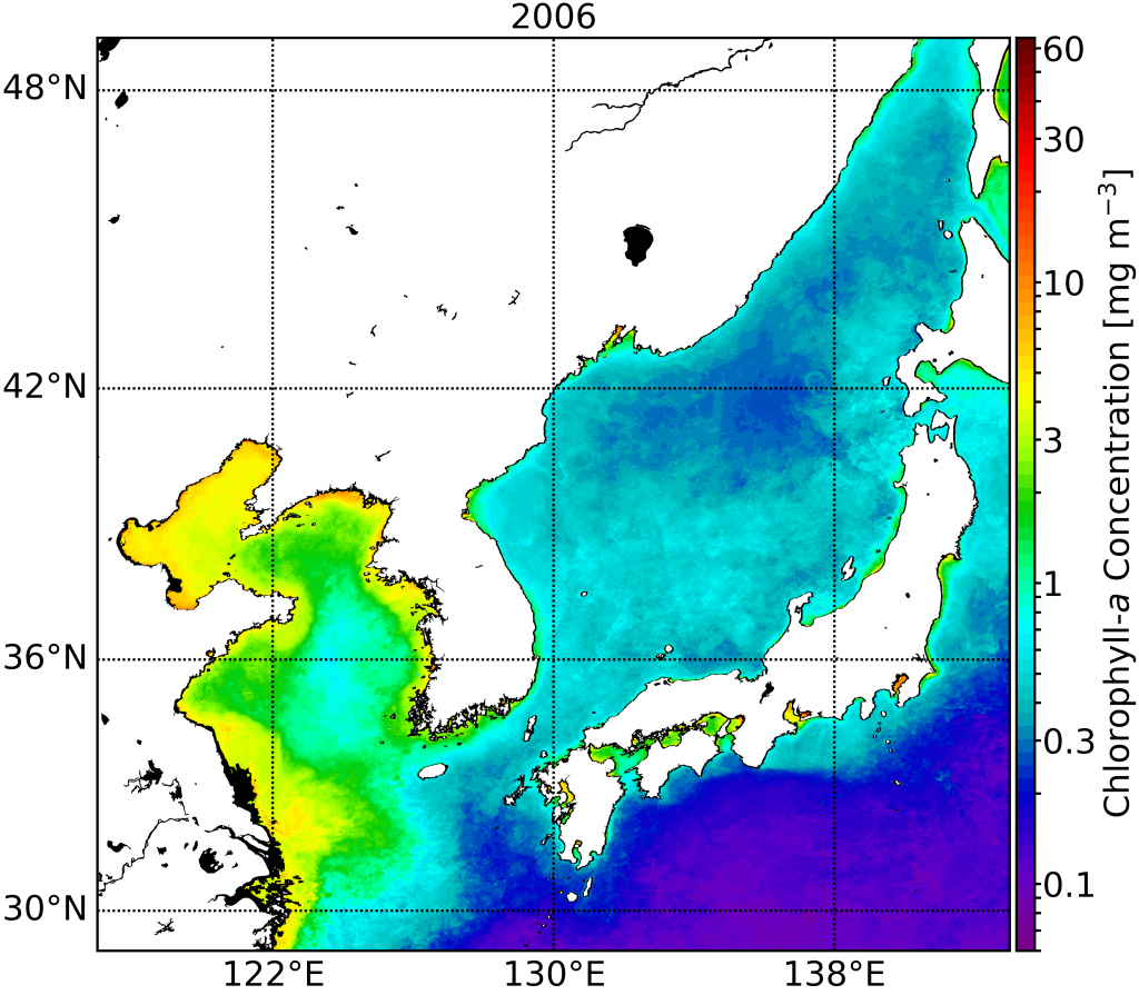
Figure 1. Sample of the CHL product provided by the NMEW (MODIS-Aqua annual composite in 2006).

1.3.2 Geophysical variables and satellite sensors

The NMEW serves as the NOWPAP’s region Distributed Active Archive Centre (DAAC) for Marine Environmental Protection of Northwest Pacific region (NW) and it provides physical and biological parameters of marine environment observed by satellite sensors in the NW.

Available biological parameters include the standard sea surface chlorophyll-a (CHL) as retrieved from the space agencies and the blended CHL, which is based on a combination of the standard algorithms from space agencies and the algorithm developed in the Yellow Sea Large Marine Ecosystem’s project on Ocean Color (YOC algorithm) (section 3.3 for more details); the total suspended matter (TSM) and the coloured dissolved organic matter (CDOM).

As for the physical parameters only the sea surface temperature (SST) is distributed. Below is a summary of the sensors from which the above datasets are obtained.

Table 1. List of primary geophysical variables retrieved by NPEC, their satellite missions, lifespan and the mission’s space agencies.

Geophysical variables	Satellite mission	Mission lifespan	Space Agency
CHL	OCTS	1996-10-31 to 1997-06-29	JAXA (Formerly NASDA)
	SeaWiFS	1997-09-04 to 2010-12-11	NASA
	MERIS	2002-03-21 to 2012-05-09	ESA
CHL & SST	MODIS-Aqua	2002-07-04 to present	NASA
CHL & SST	VIIRS-SNPP	2012-01-02 to present	NASA/NOAA
CHL, CDOM, TSM & SST	SGLI	2017-12-23 to present	JAXA
SST	AVHRR Pathfinder	1985-08-25 to present	NOAA

1.3.3 Geophysical Variables and Application Examples

a) Chlorophyll-a Concentration (CHL)

Satellite observations of CHL [mg m−3] began in 1978 with the launch of the Coastal Zone Colour Scanner (CZCS), the first satellite with ocean colour sensors (O’Reilly and Werdell, 2019) and continues to date with the sensors launched in later years as exemplified in Table 1. CHL is inarguably one of the most widely used biological parameters, often used as a proxy for phytoplankton biomass. Phytoplankton are micro autotrophs at the base of the ocean food web with major role in primary production and oxygen generation in aquatic systems. Most phytoplankton, in contrast to land plants, are buoyant and floating in the upper illuminated part of the ocean.

The applications of satellite CHL include, but not limited to, studies of ocean primary production (Chavez et al., 2010; Yamada et al., 2005), of ocean biological pump (Omand et al., 2015; Thomsen et al., 2017), of phytoplankton seasonality and fisheries (Kodama et al., 2018; Platt et al., 2003), of the ocean physical-biological interactions (Maúre et al., 2018, 2017; McGillicuddy, 2016), of climate change and variability (Cianca et al., 2012; Racault et al., 2012, 2017), of water quality assessment and monitoring assessment (Terauchi et al., 2018, 2014; Yang et al., 2018), etc. Our use of CHL at the NPEC is more focusing on the latter where we use a long-term CHL for the assessment of eutrophication in the coastal waters around the NOWPAP region (Terauchi et al., 2018). The above examples clearly showcase the importance of CHL for improved understanding of the ocean under the changing climate.

b) Coloured Dissolved Organic Matter (CDOM)

CDOM [m—1] is estimated from the SGLI/GCOM-C observations and defined as the light absorption coefficient of organics dissolved in surface water at 412 nm wavelength (Smyth et al., 2006). It is also a key indicator in water quality monitoring (Kutser et al., 2005). It is essential for understanding biogeochemical processes and ecosystem dynamics in marine waters. CDOM absorbs light and more effectively in the short wavelengths (Yang et al., 2018). Thus, it affects light availability for primary productivity. Moreover, some of the major sources of CDOM in the ocean are detritus of terrestrial plants washed by rivers and discharge in the coastal waters. Therefore, it can also be used as an important parameter that links human activities on land and the impact on coastal waters (Bai et al., 2013).

c) Total Suspended Matter (TSM)

TSM [g m—3] as estimated from the SGLI/GCOM-C observations is the dry weight of suspended matter in a unit volume of surface water constituting the sum of organic and inorganic matter such phytoplankton and soil, respectively (Toratani et al., 2012). TSM is another key water quality indicator and one of the most visible indicators of water quality. TSM can derive from soil erosion, river discharges, stirred bottom sediments or from phytoplankton (Yang et al., 2018). Excessive TSM can, among others, impair water quality for aquatic life, impede navigation and increase flooding risks (Wood, 2014). Thus, TSM is an important component of water quality monitoring.

d) Sea Surface Temperature (SST)

SST [⁰C] is an important geophysical parameter responsible for the regulation of many physical and biological processes in the ocean (Merlivat et al., 2015). SST from satellite observations is often denoted skin SST as it is an estimate of the very surface layer (～1 mm) and on average, is generally 0.1⁰ to 0.2 ⁰C cooler than the bulk surface temperature as measured by buoys and other in situ techniques (Casey and Cornillon, 1999). SST is a fundamental variable in understanding, monitoring and predicting the dynamics of the oceans and ocean-atmosphere coupling responsible for the regulation of physical-biological dynamics including primary production and air-sea fluxes of heat, momentum and gas at a variety of scales (Behrenfeld et al., 2006; Racault et al., 2017; Small et al., 2008; Tomita et al., 2019). Moreover, it is extensively used in various operational applications as in ecosystem assessments, climate change studies, fisheries, etc.

1.3.4 Spatial and Temporal Resolutions of the Data Products

The NPEC (http://www.npec.or.jp/en/) processes satellite data from Earth-viewing satellites for the NOWPAP region. These data are obtained from space agencies listed in the Table 1. Table 2 shows the spatial and temporal resolution of the available data products.

Table 2. Spatial and temporal resolutions of the data products provided in the NMEW website.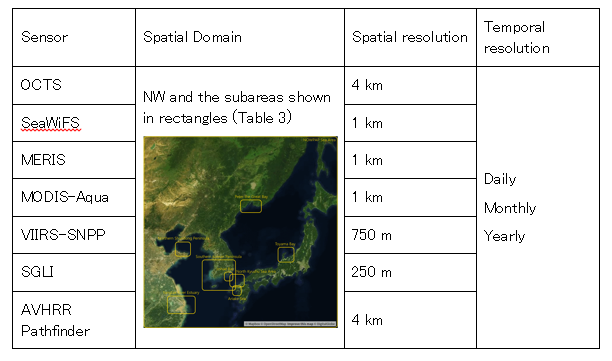

2. Data Product Format

2.1 Overview

The satellite data provided in the NMEW are Level-3 and Level-4 products. Details of the differences in the data levels can be found in later parts (section 3). All processed data are stored in a widely used libraries for data storage, namely, netCDF-4 and PNG formats. The former contains the actual processed data with the corresponding metadata while the latter are generated for quick look. The netCDF format is an open format, machine-independent, self-describing, binary data format standard for the exchange of scientific data (http://www.unidata.ucar.edu/software/netcdf).

Each data product is stored in a single netCDF file which includes the dimensions, variables, variable attributes, and global attributes (section 5). In the case of monthly/yearly composites, an additional variable (valid_pixel_count) is included and it contains the count of pixels contributing to the composite in days/months.

2.1.1 Naming Convection

The basic naming convention for the files in NMEW is as follows.
Daily composite files: iyyyymmdd_vvv_sba_tc.ext
Monthly composite files: iyyyymm_vvv_sba_tc.ext
Yearly composite files: iyyyy_vvv_sba_tc.ext

where i is the initial of the sensor with O for OCTS, S for SeaWiFS, M for MERIS, A for MODIS-Aqua, V for VIIRS-SNPP, P for AVHRR-Pathfinder, and GS for SGLI/GCOM-C. Currently OLCI data are not provided. When these data become available, the initials must be differentiated from O of OCTS in the case of OLCI. The blended CHL data has Y as the initial.

yyyymmdd corresponds to year (yyyy), month (mm) and day (dd). vvv is the data variable, CHL, CDOM, SST, and TSM.

sba indicates the subarea, for example, NW for the NOWPAP Sea Area (Table 3). tc corresponds to the temporal composite period (day, month, year).

ext indicates the file extension (nc for netCDF and png for PNG files)

Table 3. Names of the subareas for which data subset data are processed

Subarea acronym	Subarea name
NW	NOWPAP Sea Area
AS	Ariake Sea
JB	Jinhae Bay
KS	North Kyushu Sea Area-Genkai Sea
PB	Peter the Great Bay
SP	Northern Shandong Peninsula
SS	Southern Korean Peninsula
TB	Toyama Bay
YR	Yangtze River Estuary

3. Data Processing

Satellite observations come in different processing levels starting from 0, which is the unprocessed instrument/payload data at full resolution. More details on different processing levels can be obtained from space agencies like NASA (https://oceancolor.gsfc.nasa.gov/products/). Here, NPEC’s processing starts at Level 2 (L2) and makes the processed data available in the NMEW website as L3. The L2 used in generating L3 data are obtained for the space agencies (JAXA, NASA). The MERIS L2 data is obtained from ESA is also obtained through the NASA ocean color website. From NOAA, SST is obtained as L3 (Figure 2). Before moving into the description of the data processing steps, the concepts of L3 and L4 adopted in this document are introduced in the following paragraphs.

a) Level 3 Product
The Level 3 (L3) data are derived geophysical variables that have been aggregated/projected onto a well-defined regular spatial grid over a well-defined period. These L3 products have the same resolution as the source L2 data. However, as the target map is conformal, that is, the spatial grid has constant discretization angles, but not necessarily lengths, thus the pixel area is not preserved throughout the mapping projection.

b) Level 4 Product
As defined in the NASA website, Level 4 (L4) data are model output or results from analyses of lower level data (e.g., variables derived from multiple measurements). The blended CHL product (the YOC in the NMEW) make part of this level as it is a combination of CHL from different sensors and is generated through statistical analysis and the use of empirically tuned local algorithm (Siswanto et al., 2011).

3.1 Daily Screening and Mapping of Ocean Colour Data

As mentioned above, the data processing of the NMEW starts with the retrieval of the L2 data from space agencies (Figure 2). In the processing of L2 data, several satellite swaths (passes) for the area of interest are gathered and each pass is screened based on a given quality information. The screened data are then projected onto a common grid to obtain a single image. The mapped files are then composited to obtain a daily mapped product (Figure 2).

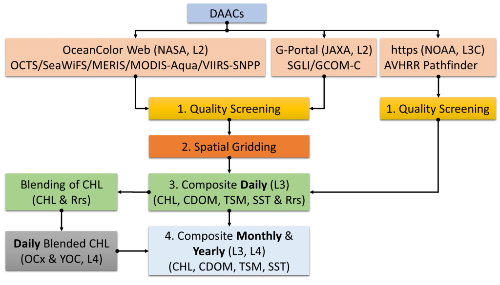
Figure 2. Outline of the data processing flow.

Screening of L2 data is based on l2_flags,one of the variables in L2 data, that contains quality of geophysical parameter information given at each pixel. The l2_flags are 16-bit array for the JAXA data, whereas they are 32-bit array for the data retrieved from NASA (Tables 4 and 5). These flags contain the conditions of each observation pixel, including the information of whether a given pixel is on land or in the ocean. The l2_flags are used to select pixels that pass into L3 products as valid against those that are discarded as invalid. The flag information is used by switching the binary digit in each of either 16 or 32-bit array to on (“1”) or off (“0”). NASA provides an interactive tool that demonstrates the concept of switching on or off the 32-bit flags (https://oceancolor.gsfc.nasa.gov/atbd/ocl2flags/).

Table 4. List of the flag bit, name, short description and screening criteria for ocean colour data obtained from NASA Ocean Color Web. These flag bits are contained in a variable named l2_flags. The TB superscript indicates the flags used for Toyama Bay (TB) subareas referring to Terauchi et al., (2014).

Bit	Name	Short Description	Flags used for screening
00	ATMFAIL^TB*	Atmospheric correction failure	Used
01	LAND^TB	Pixel is over land	Used
02	PRODWARN	One or more product algorithms generated a warning	Not Used
03	HIGLINT	Sunglint: reflectance exceeds threshold	Used
04	HILT^TB	Observed radiance very high or saturated	Used
05	HISATZEN^TB	Sensor view zenith angle exceeds threshold	Used
06	COASTZ	Pixel is in shallow water	Not Used
07	Spare
08	STRAYLIGHT	Probable stray light contamination	Used
09	CLDICE^TB	Probable cloud or ice contamination	Used
10	COCCOLITH	Coccolithophores detected	Used
11	TURBIDW	Turbid water detected	Not Used
12	HISOLZEN	Solar zenith exceeds threshold	Used
13	spare
14	LOWLW	Very low water-leaving radiance	Used
15	CHLFAIL	Chlorophyll algorithm failure	Used
16	NAVWARN	Navigation quality is suspect	Used
17	ABSAER	Absorbing Aerosols determined	Used
18	spare
19	MAXAERITER	Maximum iterations reached for NIR iteration	Used
20	MODGLINT	Moderate sun glint contamination	Not Used
21	CHLWARN	Chlorophyll out-of-bounds	Used
22	ATMWARN	Atmospheric correction is suspect	Used
23	spare
24	SEAICE	Probable sea ice contamination	Not Used
25	NAVFAIL	Navigation failure	Used
26	FILTER	Pixel rejected by user-defined filter OR Insufficient data for smoothing filter	Not Used
27	spare
28	BOWTIEDEL	Deleted off-nadir, overlapping pixels (VIIRS only)	Not Used
29	HIPOL	High degree of polarization determined	Not Used
30	PRODFAIL	Failure in any product	Not Used
31	spare

Table 5. List of the flag bit, name, short description and screening criteria for SGLI/GCOM-C ocean colour data obtained from JAXA G-Portal. *The TB superscripts indicates the flags used for Toyama Bay (TB) subareas referring to Terauchi et al., (2014).

Bit	Name	Short Description	Flags used for screening
00	DATAMISS^TB	No observation data in one or more band[s]	Used
01	LAND^TB	Pixel is over land	Used
02	ATMFAIL^TB	Atmospheric correction failure	Used
03	CLDICE^TB	Apparent cloud/ice (high reflectance)	Used
04	CLDAFFCTD^TB	Cloud-affected (near-cloud or thin/sub-pixel cloud)	Used
05	STRAYLIGHT	Stray light anticipated (atmospheric corr. abandoned) (ref. L1B stray light flags & image)	Used
06	HIGLINT^TB	High sun glint predicted (atmospheric corr. abandoned)	Used
07	MODGLINT	Moderate glint predicted (correction applied)	Not Used
08	HISOLZ^TB	Solar zenith larger than threshold	Used
09	HITAUA	Aerosol optical thickness larger than threshold	Not Used
10	NEGNLW	Negative nLw in one or more bands	Not Used
11	TURBIDW	Turbid Case 2 water,	Not Used
12	SHALLOW	Shallow water than threshold	Not Used
13	ITERFAILCDOM	Iteration failure for CDOM algorithm	Used only for CDOM
14	CHLWARN	Chlorophyll-a estimate out of range	Not Used
15	SPARE

SThe SST data follows a different processing procedure; the data are obtained as both L2 (MODIS-Aqua, VIIRS-SNPP, and SGLI/GCOM-C) and L3 (AVHRR-Pathfinder). The latter comes on a regular latitude/longitude grid, and is only quality controlled to eliminate pixels denoted as low quality (Figure 2, section 3.2).

Level 2 data of ocean colour (OC) sensors are processed to make daily composite of CHL, CDOM, SST, TSM data products. And a select of Remote Sensing Reflectance (Rrs) bands are (Table 6) used in estimating CHL based on a combination of the standard algorithms (as retrieved from space agencies, Ocx) and a regionally tuned algorithm that attempts to reduce the overestimation of CHL in the Bohai, Yellow and East China Seas (YOC, section 3.3).

Table 6. List of Rrs bands for YOC dataset in each mission in the MEW.

Sensor	Rrs bands (nm)
SeaWiFS	412, 443, 490, 555
MERIS	413, 443, 490, 560
MODIS-Aqua	412, 443, 488, 547

OC Sensors such as MODIS-Aqua, VIIRS-SNPP or SGLI/GCOM-C are still operational. In this case, obtained images are updated on daily basis. However, this process has a time lag of 1 to 2 days from the present day, meaning that, the day before the current will be available in the NMEW web.

Daily screened and mapped data are saved as netCDF and PNG (except for Rrs which are only saved as netCDF) files. Each daily composite image is saved in these formats for many subset areas as shown in Table 3.

3.2 Screening of SST

The NMEW provides different infrared-based SST products, the main difference being generally the spatial resolution. SGLI/GCOM-C is provided at 250 m, VIIRS-SNPP at 750 m, MODIS-Aqua at 1 km and AVHRR-Pathfinder provided at 4 km spatial resolution. AVHRR-Pathfinder has longer timeseries compared to the other SST products, however, the latency is large. The most recent AVHRR-Pathfinder SST has a 3-month lag.

Although the SST data from MODIS-Aqua and VIIRS-SNPP are also obtained as L2 data, they are screened based on sst_qual information, instead of the l2_flags described in the Table4. The sst_qual provide flag_masks ranging from 0 to 4 with 0 meaning BEST and 4 NOT PROCESSED or LAND. Here, GOOD quality (equivalent to 1) is selected. Below 1 is 2 which stands for QUESTIONABLE quality. Selecting GOOD (1) instead of BEST (0), more valid and useful pixels can be retrieved as 0 eliminates most of the useful pixels.

The SST data from AVHRR-Pathfinder is downloaded as L3 gridded data known as L3C (Level 3 collated) and only screened to eliminated pixels deemed invalid (Figure 2). This data come with six levels of quality thresholds (0 to 5), in reverse order of MODIS-Aqua and VIIRS-SNPP, that is, 0 means NO DATA and 5 corresponds to the BEST available SST quality. In this processing, quality threshold 4 (ACCEPTABLE QUALITY) is applied to avoid elimination or too much masking of useful pixels.

The SGLI/GCOM-C SST products are screened based on l2_flags and the flag set for this SST processing is shown in the Table 7 below.

Table 7. List of the flag bit, name, short description and screening criteria of the l2_flags for SGLI/GCOM-C SST data obtained from JAXA G-Portal.

Bit	Name	Short Description	Flags used for screening
00	No data	No data	Used
01	LAND	Pixel is over land	Used
02	REJECTED_BY_QC	Rejected by QC	Used
03	Retrieval error	Retrieval error	Not Used
04	No data (TIR1)	No data (TIR1) (TIR=thermal infrared)	Not Used
05	No data (TIR2)	No data (TIR2)	Not Used
06	Spare
07	Spare
08	0: nighttime or no visible data, 1: daytime	0: Nighttime or no visible data 1: Daytime	Not Used
09	Spare	No
10	Spare	No
11	Unknown (clear/cloudy)	Unknow (clear/cloudy)	Not Used
12	Cloudy	Cloudy	Used
13	Acceptable (possibly cloudy)	Acceptable (possibly cloudy)	Not Used
14	Good	Good	Not Used
15	Unreliable	0: Unreliable (inland/too close to land) 1: reliable	Used (when it is “0”)

3.3 The Blended CHL Dataset

The blended CHL dataset is a combined CHL from the standard and YOC-based CHL algorithms. This dataset is used for long-term change monitoring of marine environment in the NOWPAP region. The name “YOC” is derived from Yellow Sea Large Marine Ecosystem’s project on Ocean Color. The YOC algorithm is applied in the estimation of CHL in the western half of the NOWPAP sea area, that is, the Bohai, Yellow and East China Seas, where the algorithm was developed. In the eastern part, mostly in the Japan Sea, the standard algorithm is used. The YOC and the OC standard algorithms for CHL are detailed in the following sub-chapter.

3.3.1 YOC Algorithm Description

The YOC algorithm was developed by Siswanto et al. (2011) for the East China Sea region with high CDOM (coloured dissolved organic matter) and TSM (suspended sediments). The shape of the algorithm is a Tassan-like (Siswanto et al. 2011 and Tassan 1994) algorithm defined as follows.

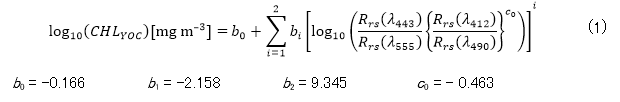
Eq. (1) was originally developed with the SeaWiFS Reprocessing 5.1 (R2005) dataset. However, current data set is reprocessing 2018 (R2018). The coefficients in Eq. (1) are updated version, as per (Yamaguchi et al., 2013), of the original Siswanto et al. (2011).

3.3.2 The OC Standard CHL algorithm Description

The OC standard CHL products combine two empirical algorithms, the Hu colour index (CI, Eq. (2)) and the O’Reilly band ratio (OCx, Eqs. (3)–(6)) algorithms (Hu et al., 2012; O’Reilly et al., 1998), . The CI algorithm is a three-band reflectance difference algorithm employing the difference between Rrs in the green band and a reference formed linearly between Rrs in the blue and red bands, Eq. (2).

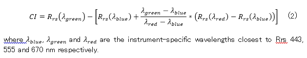
The OCx algorithms are a fourth-order polynomial empirical relationship between a ratio of Rrs and CHL. Currently, as of April 2020, the shapes of the standard algorithms (Hu et al., 2012; Morel and Maritorena, 2001; O’Reilly et al., 1998) as well as the coefficients ai (i = 0, 1, 2, 3, 4) are those shown in Eqs. (3)–(6) and Table 8. For chlorophyll retrievals below 0.15 mg m-3, the CI algorithm is used. For chlorophyll retrievals above 0.2 mg m-3, the OCx algorithm is used. In between these values, the CI and OCx algorithm are blended using a weighted approach as per NASA.

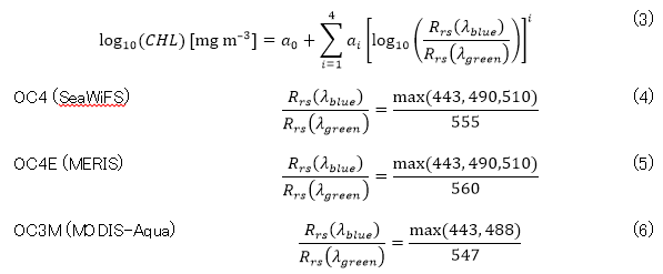
Table 8. List of the NASA default coefficients for their standard algorithms (https://oceancolor.gsfc.nasa.gov/atbd/chlor_a/). The table only includes sensors used in estimating the blended CHL product.

Sensor	Blue	Green	a₀	a₁	a₂	a₃	a₄
SeaWiFS	443>490>510	555	0.3272	-2.9940	-2.7218	-1.2259	-0.5683
MERIS	443>490>510	560	0.3255	-2.7677	2.4409	-1.1288	-0.4990
MODIS-Aqua	443>488	547	0.2424	-2.7423	1.8017	0.0015	-1.2280

The YOC algorithm follows a similar approach to NASA standard CHL product. It combines the YOC derived CHL based on Eq. (1) and standard CHL, Eq. (3). However, the switching between the YOC and the standard CHL is based on the normalised water-leaving radiance at 555 nm (nLw555, mW cm–2 µm–1 sr–1) as the focus is on turbid versus non-turbid waters. nLw555 < 1.5 defines non-turbid, whereas nLw555 > 2.5 defines turbid. In between these values (1.5 ≤ nLw555 ≤ 2.5) CHL is blended based on a linearly weighted approach (Yamaguchi et al. 2013). Further details of the computation of the YOC-based CHL are available from other works (Siswanto et al., 2011; Terauchi et al., 2018; Yamaguchi et al., 2013).

3.4 Temporal Composite

The data in the NMEW are provided in different temporal resolutions, namely daily, monthly, and yearly composites (Figure 2). Monthly composites are generated from the daily and the yearly from monthly composites. Monthly (Yearly) netCDF files contain a variable with the number of pixels (valid_pixel_count) contributing to the composite at the pixel level, that is, number of days (months).

4. HOW To

4.1 Access the NMEW Data

The NMEW website provides two basic ways of searching, visualising and downloading the data; the Data Search (DS, https://ocean.nowpap3.go.jp/image_search/) and Sea Calendar (SC, https://ocean.nowpap3.go.jp/image_search/?latest). DS and SC are basically the same except that SC by default opens the latest calendar month and fills in pre-defined parameters. More details on DS and SC in 4.1.1 and 4.1.2. The data at the NMEW are provided in different temporal resolutions, namely, daily, monthly, and yearly composites. The spatial resolution is the same as the original source data, that is, if an ocean colour instrument observes the ocean at spatial resolution of 1 km, the NMEW also provides the processed information at the same resolution of 1 km. It is worth noting, however, that 1 km is mostly the nadir resolution and it decreases away from the swath centre.

4.1.1 The Data Search Interface

Through the Data Search (DS) interface—the search criteria—it is possible to custom select the display sensor, data product (variable of interest), sub areas (each of the 8 plus the whole NW, as shown by the yellow boxes in Figure 3), the composite period and visualisation/download time (Date Range). The Year and Month in the Date Range along with the Daily Composite in the Period panel are useful in displaying daily composites of a given calendar month. When “Monthly, Yearly Composite” panel is selected, the Date Range disables Month and only Year becomes selectable. This option allows the visualization of a total of 7-year period centred on the currently selected year. That is, if 2017 is selected, monthly and yearly composites of 2014 through 2020 will be displayed. However, it is important to note this window of 3-year before and after the currently selected year (e.g. 2017) depends on data availability.

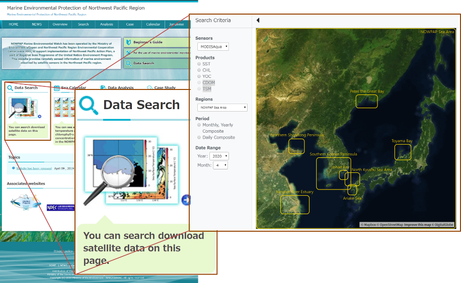
Figure 3. Outline of the data search in the NMEW website.

4.1.2 The Sea Calendar Interface

Unlike the DS in which a manual selection by the user is necessary, the Sea Calendar (SC) does an automatic custom selection using a pre-defined setting. In the current setting (as of April 2020), it defaults to MODIS-Aqua for the Sensors, CHL for the Products, NW for Regions, Daily Composite for the Period, and current year, and month for the Date Range. The images outside the selected month are grey-shaded as shown in the Figure 4, example in April 2020.

Similar to the grey-shaded days outside the currently selected month, any product not available from the selected sensor is also greyed-out. This procedure also applies to the Date Range where years before and after the lifespan of a given sensor are greyed-out. In the Products field, YOC is the only one selectable independently of the sensor selection as it is sensor-independent product (see section 3.3).

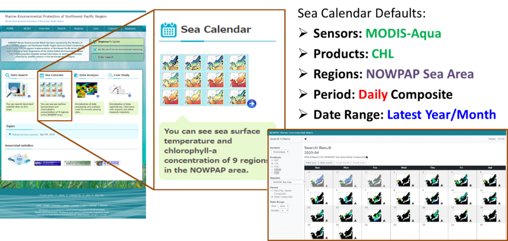
Figure 4. Same as Figure 3 but for sea calendar.

4.2 Bulk Data Download

While it is possible to interactively download the data based on the methods introduced above, the NMEW website does not currently provide a method, like as FTP (File Transfer Protocol) for instance, for bulk download of the data. Instead, here we introduce an alternative way to download as much data as needed using a script based on the open source Python programming language (https://www.python.org/). The method is simple and uses the requests (https://requests.readthedocs.io/en/master/) module. We assume a basic understanding of the Python language and only provide a code snippet for demonstration purposes.

The example shows how to download monthly CHL data and quick look image files for the NW region from 1998 to 2005 for the SeaWiFS sensor. Based on the example (Figure 5), any subarea or date range can be customised to user needs.

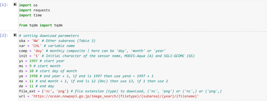
Figure 5. Example of parameter setup for bulk downloading of the NMEW data products using Python’s requests module. Cell [1] imports the modules to be used, and [2] set some parameters for data download

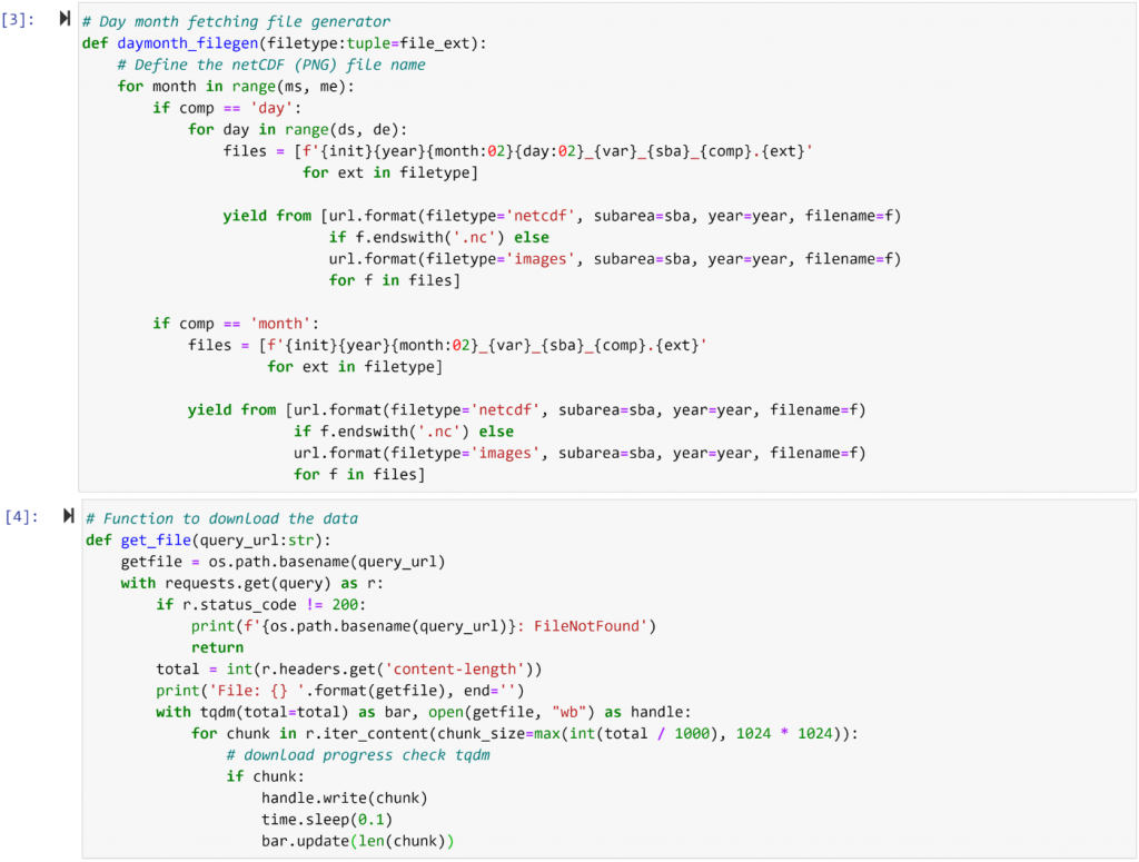
Figure 6. Function definitions (following Figure 5) to be used in bulk download example. Cell [3] defines the function that generates the file to be downloaded, whereas [4] defines the function that downloads the generated file.

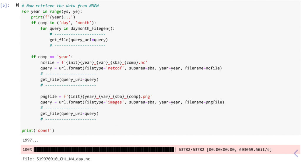
Figure 7. Code cell that runs the actual download. It distinguishes the downloads based on composite period (daily, monthly, or yearly) as they all have different file patterns. This cell calls functions in Figure 6 to generate file names and download URLs (Uniform Resource Locator, the address of a World Wide Web page) based on parameters set in cell [2] (Figure 5). Then, it saves one file at a time in the current working directory. As the files are being downloaded, below the cell, the progress of downloads will be displayed. When all is complete, the cell prints “done!”. The Python script for this example can be obtained freely from https://github.com/npec/NMEW.demos/blob/master/NMEW_bulk_download_demo.py

4.3 Read the Data

Data available through the NMEW website may be read by means of netCDF library (https://www.unidata.ucar.edu/software/netcdf/) or any third-party tool capable of reading netCDF files (e.g. WIM, https://www.wimsoft.com/). NetCDF is a convenient, standard, self-describing, and platform independent format for data transport.

SST data are stored as integer values. They can be converted back into geophysical values using the relation SST = sst * scale_factor + add_offset.

The scale_factor and add_offset is stored in the attributes of the sst product of the netCDF. A standard netCDF library does as automatic conversion of the data using the equation above. Moreover, it also masks the data based on _FiilValue or missing_value if these fields are set in the attributes of the variable. CHL, CDOM and TSM are stored as floating numbers and they do not require any conversion.

4.4 Visualise the Data

All NMEW products are mapped on a regular latitude/longitude grid so they can easily be visualised using specialised tools. In the following example, we demonstrate how the data can be visualised using Python.

We will use a monthly file of CHL from April 2020, NW and use the netCDF4, matplotlib, and Basemap modules for data display. Basemap is optional and is used for working with geographic data (map projection, drawing of coastlines, etc.). We demonstrate the visualisation with and without the use of Basemap.

The code snippet goes through the details to visualise the data. [1] through [3] import modules, set some basics visualisation parameters, and read the dataset using the netCDF library (Figure 8). [4] display a image using the imshow function from matplotlib (Figure 9 and Figure 10), whereas [5] uses pcolormesh and Basemap (Figure 11 and Figure 12). Basemap handles the filling of land, coastlines, and ocean. In general, from [4] we cannot distinguish the land from missing pixels in the ocean unless we use a mask that clearly distinguishes these two, whereas from [5] is quite simple as we can set different filling colours for land versus ocean by simply relying on Basemap. For details, see the code snippet below and the respective figures.

It is worth noting although Basemap is a great tool for creating maps using Python in a simple way (https://basemaptutorial.readthedocs.io/en/latest/index.html), its deprecation has been announced. CartoPy (https://scitools.org.uk/cartopy/docs/latest/) is designated to replace Basemap. However, Basemap still offers a powerful way to work with geospatial data.

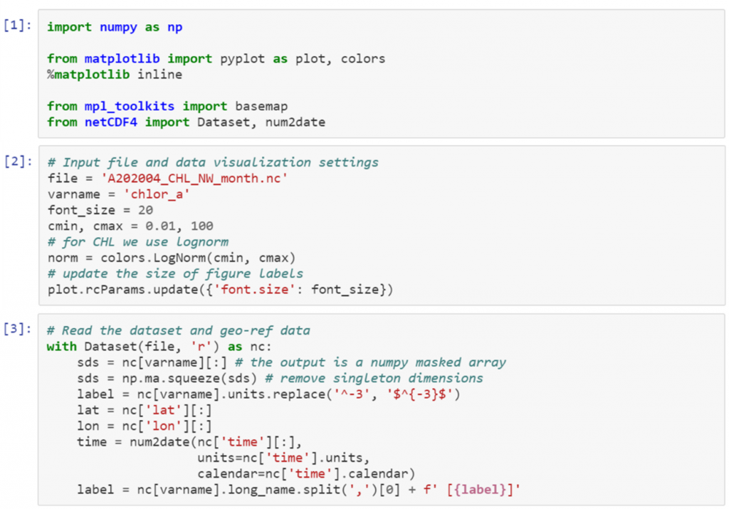
Figure 8. Visualisation setup for the NMEW products using Python’s matplotlib module. Cell [1] imports the modules to be used, [2] set some parameters for data visualisation, and [3] reads the data, time, geolocation, and labels.

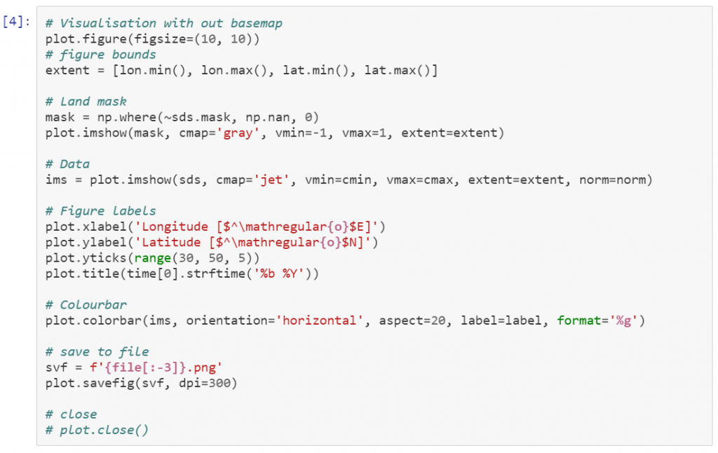
Figure 9. Visualisation of NMEW products (CHL) using imshow function of the matplotlib module.

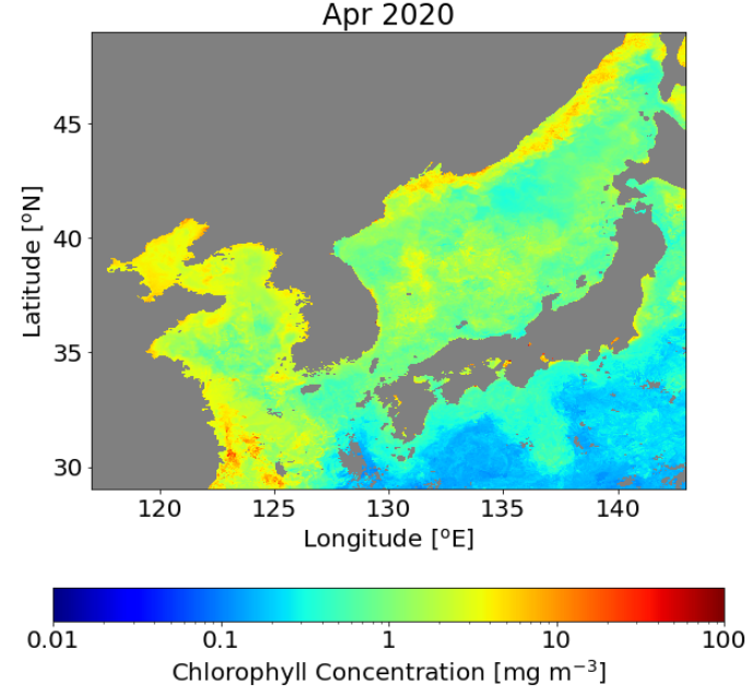
Figure 10. Visualisation of NMEW products (CHL) generated by the code snippet in Figure 9

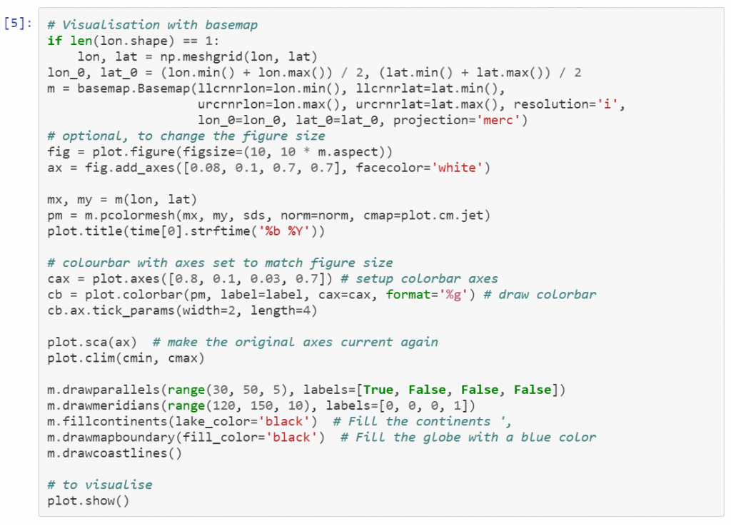
Figure 11. Same as in Figure 9 but with the use of pcolormesh and Basemap modules as opposed to imshow function.

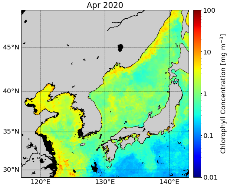
Figure 12. Visualisation of NMEW products (CHL) generated by the code snippet in Figure 11Figure .

5. NetCDF File Structure

NetCDF (Network Common Data form) is a set of software libraries and machine-independent data formats that support the creation, access, and sharing of array-orriended scientific data. Below is an example of the output of netCDF library command ncdump -h filename, where filename is replaced by the input file, in this case A202004_CHL_NW_month.nc. The command outputs the file structure information of the netCDF file as shown below.

netcdf A202004_CHL_NW_month {
dimensions:

time = 1 ;
lat = 2219 ;
lon = 2250 ;

variables:

int time(time) ;

time:standard_name = “time” ;
time:long_name = “reference time of the monthly composite file” ;
time:axis = “T” ;
time:units = “seconds since 1981-01-01 00:00:00” ;
time:calendar = “gregorian” ;

int crs ;

crs:standard_name = “coordinate reference system” ;
crs:grid_mapping_name = “custom_latitude_longitude_grid” ;
crs:dx = 0.0115509f ;
crs:dy = -0.009010315f ;
crs:lat = “lat_max:dy:(lat_max-dy)+dy*lat_size” ;
crs:lon = “lon_min:dx:(lon_min-dx)+dx*lon_size” ;
crs:comment = “This variable only contains the description of the grid_mapping” ;

float lat(lat) ;

lat:standard_name = “latitude” ;
lat:long_name = “latitude” ;
lat:units = “degrees_north” ;
lat:grid_mapping = “crs” ;
lat:axis = “Y” ;
lat:valid_min = 29.01117f ;
lat:valid_max = 48.99549f ;

float lon(lon) ;

lon:standard_name = “longitude” ;
lon:long_name = “longitude” ;
lon:units = “degrees_east” ;
lon:grid_mapping = “crs” ;
lon:axis = “Y” ;
lon:valid_min = 117.0058f ;
lon:valid_max = 142.9894f ;

float chlor_a(time, lat, lon) ;

chlor_a:long_name = “Chlorophyll Concentration, OCI Algorithm” ;
chlor_a:standard_name = “mass_concentration_of_chlorophyll_in_sea_water” ;
chlor_a:units = “mg m^-3” ;
chlor_a:_FillValue = -32767.f ;
chlor_a:grid_mapping = “crs” ;
chlor_a:valid_min = 0.09948392f ;
chlor_a:valid_max = 97.58238f ;
chlor_a:reference = “Hu, C., Lee Z., and Franz, B.A. (2012). Chlorophyll-a algorithms for oligotrophic oceans: A novel approach based on three-band reflectance difference, J. Geophys. Res., 117, C01011, doi:10.1029/2011JC007395.” ;
short valid_pixel_count(time, lat, lon) ;
valid_pixel_count:standard_name = “count of valid pixels” ;
valid_pixel_count:long_name = “number of valid data in each pixel for the 　composite period” ;
valid_pixel_count:units = “count” ;
valid_pixel_count:_FillValue = -32767s ;
valid_pixel_count:valid_min = 1s ;
valid_pixel_count:valid_max = 16s ;

}

// global attributes:

:product_name = “A202004_CHL_NW_month.nc” ;
:title = “MODISA Level-2 chlor_a screened for bad pixels” ;
:platform = “Aqua” ;
:instrument = “MODIS” ;
:processing_level = “L3” ;
:temporal_range = “month (30-days)” ;
:time_coverage_start = “20200401T000000Z” ;
:time_coverage_end = “20200430T000000Z” ;
:processing_version = “2018.1QLP” ;
:input_files = “A20200401_CHL_NW_day.nc; A20200402_CHL_NW_day.nc; A20200417_CHL_NW_day.nc; A20200422_CHL_NW_day.nc; A20200424_CHL_NW_day.nc; A20200418_CHL_NW_day.nc; A20200419_CHL_NW_day.nc; A20200420_CHL_NW_day.nc; A20200421_CHL_NW_day.nc; A20200423_CHL_NW_day.nc; A20200403_CHL_NW_day.nc; A20200425_CHL_NW_day.nc; A20200404_CHL_NW_day.nc; A20200426_CHL_NW_day.nc; A20200427_CHL_NW_day.nc; A20200405_CHL_NW_day.nc; A20200428_CHL_NW_day.nc; A20200406_CHL_NW_day.nc; A20200429_CHL_NW_day.nc; A20200407_CHL_NW_day.nc; A20200408_CHL_NW_day.nc; A20200430_CHL_NW_day.nc; A20200409_CHL_NW_day.nc; A20200410_CHL_NW_day.nc; A20200411_CHL_NW_day.nc; A20200412_CHL_NW_day.nc; A20200413_CHL_NW_day.nc; A20200414_CHL_NW_day.nc; A20200415_CHL_NW_day.nc; A20200416_CHL_NW_day.nc” ;
:l2_flags = “ATMFAIL, LAND, HIGLINT, HILT, HISATZEN, STRAYLIGHT, CLDICE, COCCOLITH, HISOLZEN, LOWLW, CHLFAIL, NAVWARN, ABSAER, MAXAERITER, ATMWARN, NAVFAIL” ;
:spatial_resolution = “1.0 km” ;
:latitude_step = 0.009010315f ;
:longitude_step = 0.0115509f ;
:geospatial_lon_min = 117LL ;
:geospatial_lon_max = 143LL ;
:geospatial_lat_min = 29LL ;
:geospatial_lat_max = 49LL ;
:date_created = “Sat May 2 10:26:17 2020” ;
:subarea = “nowpap_sea_area” ;
:project = “Northwest Pacific Action Plan” ;
:creator_name = “UNEP > NOWPAP > CEARAC” ;
:creator_url = “http://cearac.nowpap.org” ;
:creator_email = “webmaster@cearac.nowpap.org” ;
:publisher_name = “Marine Environmental Protection of Northwest Pacific Region” ;
:publisher_url = “https://ocean.nowpap3.go.jp/” ;

6. Acknowledgement

In your use of the products downloaded from the Marine Environmental Watch website (https://ocean.nowpap3.go.jp/), please acknowledge the Northwest Pacific Region Environmental Cooperation Center (NPEC, http://www.npec.or.jp/en/) for preparing and providing data for the NOWPAP region. For inquiries, please contact us at terauchi@npec.or.jp. Example for general acknowledgement is provided below.

The chlorophyll a and sea surface temperature products were provided by the NPEC (http://www.npec.or.jp/en/) funded by the Ministry of Environment of Japan for Environmental Monitoring (https://ocean.nowpap3.go.jp/) of the Northwest Pacific region.

7. References

Bai, Y., Pan, D., Cai, W.J., He, X., Wang, D., Tao, B., Zhu, Q., 2013. Remote sensing of salinity from satellite-derived CDOM in the Changjiang River dominated East China Sea. J. Geophys. Res. Ocean. 118, 227–243. https://doi.org/10.1029/2012JC008467

Behrenfeld, M.J., O’Malley, R.T., Siegel, D.A., McClain, C.R., Sarmiento, J.L., Feldman, G.C., Milligan, A.J., Falkowski, P.G., Letelier, R.M., Boss, E.S., 2006. Climate-driven trends in contemporary ocean productivity. Nature 444, 752–755. https://doi.org/10.1038/nature05317

Casey, K.S., Cornillon, P., 1999. A Comparison of Satellite and In Situ–Based Sea Surface Temperature Climatologies. J. Clim. 12, 1848–1863. https://doi.org/10.1175/1520-0442(1999)012<1848:ACOSAI>2.0.CO;2

Chavez, F.P., Messié, M., Pennington, J.T., 2010. Marine Primary Production in Relation to Climate Variability and Change. Ann. Rev. Mar. Sci. 3, 227–260. https://doi.org/10.1146/annurev.marine.010908.163917

Cianca, A., Godoy, J.M., Martin, J.M., Perez-Marrero, J., Rueda, M.J., Llinás, O., Neuer, S., 2012. Interannual variability of chlorophyll and the influence of low-frequency climate modes in the North Atlantic subtropical gyre. Global Biogeochem. Cycles 26, 1–11. https://doi.org/10.1029/2010GB004022

Hu, C., Lee, Z., Franz, B., 2012. Chlorophyll a algorithms for oligotrophic oceans: A novel approach based on three-band reflectance difference. J. Geophys. Res. Ocean. 117, 1–25. https://doi.org/10.1029/2011JC007395

Kodama, T., Wagawa, T., Ohshimo, S., Morimoto, H., Iguchi, N., Fukudome, K.-I., Goto, T., Takahashi, M., Yasuda, T., 2018. Improvement in recruitment of Japanese sardine with delays of the spring phytoplankton bloom in the Sea of Japan. Fish. Oceanogr. 27, 289–301. https://doi.org/10.1111/fog.12252

Kutser, T., Pierson, D.C., Tranvik, L., Reinart, A., Sobek, S., Kallio, K., 2005. Using satellite remote sensing to estimate the colored dissolved organic matter absorption coefficient in lakes. Ecosystems 8, 709–720. https://doi.org/10.1007/s10021-003-0148-6

Maúre, E.R., Ishizaka, J., Aiki, H., Mino, Y., Yoshie, N., Goes, J.I., Gomes, H.R., Tomita, H., 2018. One-Dimensional Turbulence-Ecosystem Model Reveals the Triggers of the Spring Bloom in Mesoscale Eddies. J. Geophys. Res. Ocean. 123, 6841–6860. https://doi.org/10.1029/2018JC014089

Maúre, E.R., Ishizaka, J., Sukigara, C., Mino, Y., Aiki, H., Matsuno, T., Tomita, H., Goes, J.I., Gomes, H.R., 2017. Mesoscale Eddies Control the Timing of Spring Phytoplankton Blooms: A Case Study in the Japan Sea. Geophys. Res. Lett. 44, 11,115-11,124. https://doi.org/10.1002/2017GL074359

McGillicuddy, D.J., 2016. Mechanisms of Physical-Biological-Biogeochemical Interaction at the Oceanic Mesoscale. Ann. Rev. Mar. Sci. 8, 125–159. https://doi.org/10.1146/annurev-marine-010814-015606

Merlivat, L., Boutin, J., Antoine, D., 2015. Roles of biological and physical processes in driving seasonal air–sea CO 2 flux in the Southern Ocean: New insights from CARIOCA pCO 2. J. Mar. Syst. 147, 9–20. https://doi.org/10.1016/j.jmarsys.2014.04.015

Morel, A., Maritorena, S., 2001. Bio-optical properties of oceanic waters: A reappraisal. J. Geophys. Res. Ocean. 106, 7163–7180. https://doi.org/10.1029/2000jc000319

O’Reilly, J.E., Maritorena, S., Mitchell, B.G., Siegel, D.A., Carder, K.L., Garver, S.A., Kahru, M., McClain, C., 1998. Ocean color chlorophyll algorithms for SeaWiFS. J. Geophys. Res. Ocean. 103, 24937–24953. https://doi.org/10.1029/98JC02160

O’Reilly, J.E., Werdell, P.J., 2019. Chlorophyll algorithms for ocean color sensors – OC4, OC5 & OC6. Remote Sens. Environ. 229, 32–47. https://doi.org/10.1016/j.rse.2019.04.021

Omand, M.M., D’Asaro, E.A., Lee, C.M., Perry, M.J., Briggs, N., Cetinić, I., Mahadevan, A., 2015. Eddy-driven subduction exports particulate organic carbon from the spring bloom. Science (80-. ). 348, 222–225. https://doi.org/10.1126/science.1260062

Platt, T., Fuentes-Yaco, C., Frank, K.T., 2003. Spring algal bloom and larval fish survival. Nature 423, 398–399. https://doi.org/10.1038/423398b

Racault, M., Le Quéré, C., Buitenhuis, E., Sathyendranath, S., Platt, T., 2012. Phytoplankton phenology in the global ocean. Ecol. Indic. 14, 152–163. https://doi.org/10.1016/j.ecolind.2011.07.010

Racault, M.F., Sathyendranath, S., Brewin, R.J.W., Raitsos, D.E., Jackson, T., Platt, T., 2017. Impact of El Niño variability on oceanic phytoplankton. Front. Mar. Sci. 4, 133. https://doi.org/10.3389/fmars.2017.00133

Siswanto, E., Tang, J., Yamaguchi, H., Ahn, Y.H., Ishizaka, J., Yoo, S., Kim, S.W., Kiyomoto, Y., Yamada, K., Chiang, C., Kawamura, H., 2011. Empirical ocean-color algorithms to retrieve chlorophyll-a, total suspended matter, and colored dissolved organic matter absorption coefficient in the Yellow and East China Seas. J. Oceanogr. 67, 627–650. https://doi.org/10.1007/s10872-011-0062-z

Small, R.J., DeSzoeke, S.P., Xie, S.P., O’Neill, L., Seo, H., Song, Q., Cornillon, P., Spall, M., Minobe, S., 2008. Air-sea interaction over ocean fronts and eddies. Dyn. Atmos. Ocean. 45, 274–319. https://doi.org/10.1016/j.dynatmoce.2008.01.001

Smyth, T.J., Moore, G.F., Hirata, T., Aiken, J., 2006. Semianalytical model for the derivation of ocean color inherent optical properties: Description, implementation, and performance assessment. Appl. Opt. https://doi.org/10.1364/AO.45.008116

Tassan, S. (1994). Local algorithm using SeaWiFS data for retrieval of phytoplankton pigment, suspended sediments and yellow substance in coastal waters. Appl. Optics, 12, 2369-2378.

Terauchi, G., Maúre, E. de R., Yu, Z., Wu, Z., Kachur, V., Lee, C., Ishizaka, J., 2018. Assessment of eutrophication using remotely sensed chlorophyll-a in the Northwest Pacific region, in: Frouin, R.J., Murakami, H. (Eds.), Remote Sensing of the Open and Coastal Ocean and Inland Waters. SPIE, p. 17. https://doi.org/10.1117/12.2324641

Terauchi, G., Tsujimoto, R., Ishizaka, J., Nakata, H., 2014. Preliminary assessment of eutrophication by remotely sensed chlorophyll-a in Toyama Bay, the Sea of Japan. J. Oceanogr. 70, 175–184. https://doi.org/10.1007/s10872-014-0222-z

Thomsen, L., Aguzzi, J., Costa, C., De Leo, F., Ogston, A., Purser, A., 2017. The Oceanic Biological Pump: Rapid carbon transfer to depth at Continental Margins during Winter. Sci. Rep. 7, 1–10. https://doi.org/10.1038/s41598-017-11075-6

Tomita, H., Hihara, T., Kako, S., Kubota, M., Kutsuwada, K., 2019. An introduction to J-OFURO3, a third-generation Japanese ocean flux data set using remote-sensing observations. J. Oceanogr. 75, 171–194. https://doi.org/10.1007/s10872-018-0493-x

Toratani, M., Ishizaka, J., Kiyomoto, Y., Ahn, Y.-H., Yoo, S., Kim, S.-W., Tang, J., 2012. Estimation of total suspended matter from three near infrared bands, in: Remote Sensing of the Marine Environment II. https://doi.org/10.1117/12.979669

Wood, B.M.S., 2014. Estimating suspended sediment in rivers using acoustic Doppler meters. U.S. Geol. Surv. Fact Sheet 2014-3038. https://doi.org/10.3133/fs20143038

Yamada, K., Ishizaka, J., Nagata, H., 2005. Spatial and temporal variability of satellite primary production in the Japan Sea from 1998 to 2002. J. Oceanogr. 61, 857–869. https://doi.org/10.1007/s10872-006-0005-2

Yamaguchi, H., Ishizaka, J., Siswanto, E., Baek Son, Y., Yoo, S., Kiyomoto, Y., 2013. Seasonal and spring interannual variations in satellite-observed chlorophyll-a in the Yellow and East China Seas: New datasets with reduced interference from high concentration of resuspended sediment. Cont. Shelf Res. 59, 1–9. https://doi.org/10.1016/j.csr.2013.03.009

Yang, M.M., Ishizaka, J., Goes, J.I., Gomes, H. do R., Maúre, E. de R., Hayashi, M., Katano, T., Fujii, N., Saitoh, K., Mine, T., Yamashita, H., Fujii, N., Mizuno, A., 2018. Improved MODIS-Aqua chlorophyll-a retrievals in the turbid semi-enclosed Ariake Bay, Japan. Remote Sens. https://doi.org/10.3390/rs10091335